05: Generating Estimates: Reliability and Suppression • RSTr

Overview

Though RSTr is designed to stabilize low-population regions, there is a limit to the amount of information the model can gather, and estimates from exceedingly low-population regions may be over-smoothed. To address these issues, we can establish criteria that indicate whether our estimates are reliable enough to display. In this vignette, we will take a deep dive into estimate reliability and showcase how we can use reliability criteria to suppress our estimates with suppress_estimates().

Traceplots

Let’s quickly demonstrate the importance of reliability metrics by comparing the traceplots of high- and low-population counties:

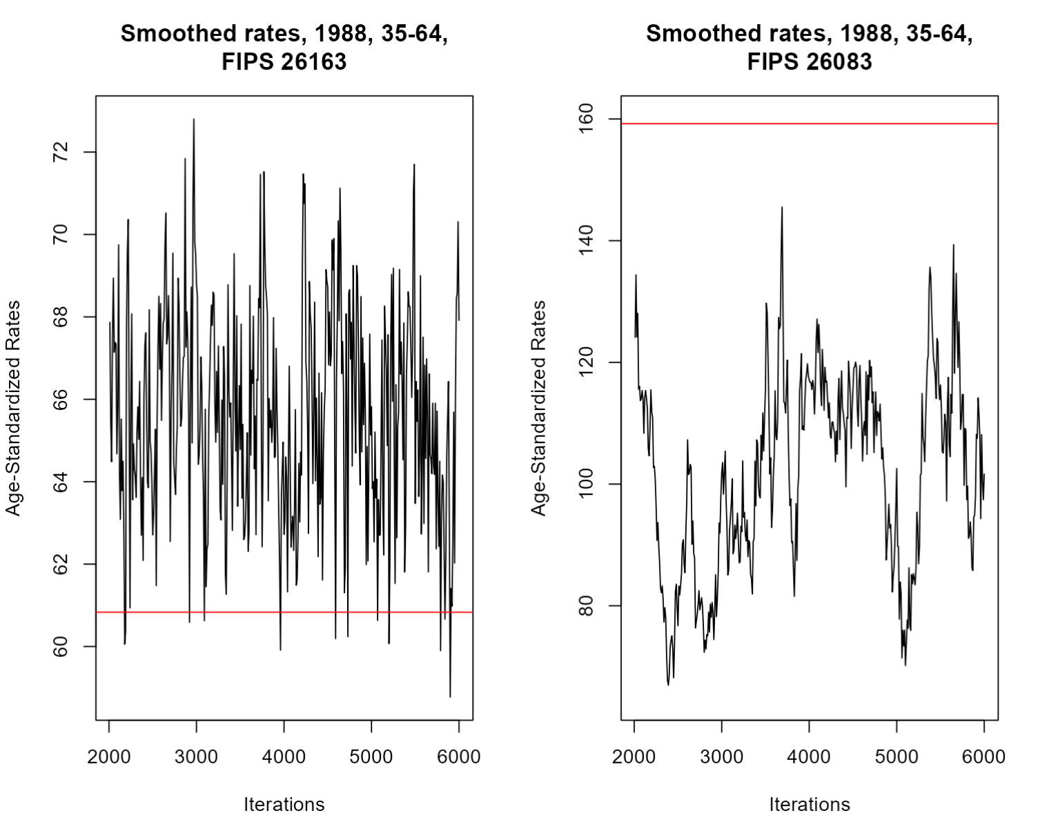
Here, we have two traceplots representing our sample values over time for a given county-group-year. On the left, we can see a traceplot for the highest-population county, and on the right is a traceplot for the lowest-population county. Each traceplot also includes a red line representing the mean event rate for that county-group-year. Note that in both traceplots, the mean line is nearby the plots, but either higher or lower than their general trend, indicating that the rates in both of these counties were attenuated thanks to spatial smoothing.

The traceplot on the left is exactly what we want to see: it is clearly fluctuating around a certain value. The right traceplot, however, is a bit less favorable: the value doesn’t seem to want to stabilize and jumps between values over the course of the model. However, the rate itself is naturally high, so the intensity of the fluctuation isn’t shocking. Smaller counties like the one shown here demonstrate the limits of RSTr: while the samples do hover around a single value for some iterations, the estimated values we would get for the county-group-year on the right will not be as reliable as estimates on the left due to the large variability of the samples gathered. Estimates like these are why we need standard measures of reliability.

Reliability can be easily tested in CAR models using two criteria:

Relative precision: In Quick, et al 2024, relative precision is measured as a ratio of the posterior median to its credible interval. If an estimate’s ratio is less than 1, then that estimate is considered unreliable at that level of credibility. Effectively, this means that unreliable estimates have a spread of samples larger than the value of the estimate itself; and
Population counts: Because of the limitations of RSTr’s models to gather information from low-population areas, estimates from any region that fall below a specified threshold will be considered unreliable, regardless of relative precision. Use your judgment when setting this threshold depending on what kind of data you are working with: for example, 1,000 population is generally a good rule of thumb for mortality data, whereas an appropriate cutoff for birth data is closer to 100. Note that this population count metric only applies for unrestricted models; the enhancements of the restricted CAR models mean that we don’t need this criterion when evaluating reliability.

Let’s get some reliability metrics for our dataset. The mstcar() function automatically generates credible intervals and relative precisions based on the perc_ci argument:

mod_mst <- mstcar(name = "my_test_model", data = miheart, adjacency = miadj, seed = 1234, perc_ci = 0.95)
#> Starting sampler on Batch 1 at Fri Dec 19 00:09:30

#> Generating estimates...
#> Model finished at Fri Dec 19 00:09:56

Here, we specify perc_ci = 0.95, which means our relative precision estimates will be based on a 95% credible interval. If we want to generate our suppressed estimates, we can simply input our RSTr model object into the suppress_estimates() function. Since we are using an MSTCAR model, we have to specify a population threshold to suppress counties with small population counts:

mod_mst <- suppress_estimates(mod_mst, threshold = 1e3)
mod_mst
#> RSTr object:
#> 
#> Model name: my_test_model 
#> Model type: MSTCAR 
#> Data likelihood: binomial 
#> Estimate Credible Interval: 95% 
#> Number of geographic units: 83 
#> Number of samples: 6000 
#> Estimates age-standardized: No 
#> Estimates suppressed: Yes 
#> Number of reliable rates: 3605 / 4980 (72.4%)
estimates <- get_estimates(mod_mst)
head(estimates)
#>   county group year  medians medians_suppressed ci_lower  ci_upper  rel_prec
#> 1  26001 35-44 1979 41.98634                 NA 29.79605  56.17417 1.5917110
#> 2  26003 35-44 1979 51.00178                 NA 37.86450 119.49006 0.6248260
#> 3  26005 35-44 1979 23.76272           23.76272 16.29719  33.58478 1.3745537
#> 4  26007 35-44 1979 33.61042           33.61042 24.15788  45.44376 1.5790005
#> 5  26009 35-44 1979 29.70584           29.70584 22.96456  39.27994 1.8207267
#> 6  26011 35-44 1979 38.17390                 NA 24.89862  65.99126 0.9289717
#>   events population
#> 1      1        964
#> 2      1       1011
#> 3      0       9110
#> 4      0       3650
#> 5      0       1763
#> 6      0       1470

By default, suppress_estimates() will suppress based on population counts, but by specifying type = "event", you can alternatively use an event count threshold. This is helpful when maintaining consistency with datasets that suppress by events instead of population, such as CDC WONDER. Notice that the first two regions in the 35-44 age group have been suppressed; the first was suppressed by population (964) and the second was suppressed by relative precision (0.925). Now, we can map out our county estimates with suppression:

library(ggplot2)
est_3544 <- estimates$medians_suppressed[estimates$group == "35-44" & estimates$year == "1988"]
ggplot(mishp) +
  geom_sf(aes(fill = est_3544)) +
  labs(
    title = "Smoothed Myocardial Infarction Death Rates in MI, Ages 35-44, 1988",
    fill = "Deaths per 100,000"
  ) +
  scale_fill_viridis_c() +
  theme_void()

These suppressed maps highlight an important benefit of age-standardizing: we can combine age groups to both bolster our relative precisions and to increase the total population in our groups, increasing values for both suppression criteria. Let’s age-standardize to 35-64 and see what counties are suppressed:

std_pop <- c(113154, 100640, 95799)
mod_mst <- age_standardize(mod_mst, std_pop, new_name = "35-64", groups = c("35-44", "45-54", "55-64"))
estimates <- get_estimates(mod_mst)

The RSTr model object remembers that we’ve suppressed our estimates and automatically performs suppression on our age-standardized estimates. Let’s map our age-standardized rates:

est_3564 <- estimates$medians_suppressed[estimates$group == "35-64" & estimates$year == "1988"]
ggplot(mishp) +
  geom_sf(aes(fill = est_3564)) +
  labs(
    title = "Smoothed Myocardial Infarction Death Rates in MI, Ages 35-64, 1988",
    fill = "Deaths per 100,000"
  ) +
  scale_fill_viridis_c() +
  theme_void()

As we increase our CI width from 0.50 to 0.95 to 0.99 and 0.995, our reliability criteria becomes more stringent and more counties become grayed out. It is important to find a good balance between credible interval choice and displaying of estimates; the traditionally-used credible interval of 95% provides a happy medium of these two factors.

Final thoughts

In this vignette, we investigated measures of reliability and observed how reliability measures change which data are suppressed. This vignette concludes the main sections on using the functions in the RSTr package. After reading these, you should be able to prepare your event and adjacency data, configure your model as necessary, age-standardize estimates, and determine which estimates are reliable. If you are interested in more advanced features of the RSTr involving sample processing, read vignette("RSTr-samples"); if you’d like more information on defining custom inits and priors, check vignette("RSTr-initialvalues") and vignette("RSTr-priors"), respectively; if you are interested in learning more about how the MSTCAR model itself works, read vignette("RSTr-models").