06: Model Informativeness • RSTr

Overview

Up to this point, we’ve discussed preparing count/adjacency data, model setup, and age-standardization. In vignette("RSTr-reliability"), we discussed how to suppress estimates based on reliability criteria, including population thresholds and relative precision. However, there are cases where the event or population counts are too low for RSTr to meaningfully gather information from neighboring regions; in these cases, the standard BYM models will apply excessive spatial smoothing, artificially inflating the estimate’s relative precision. In this vignette, we will look under the hood of the CAR models and how they perform spatial smoothing, discuss model informativeness, and how to work with restricted models in your data.

How does spatial smoothing work?

Spatial smoothing acts by way of a spatial random effects estimator Z; this is essentially the parameter that tells the model how much to either increase or decrease its corresponding estimated rate lambda. In CAR models, the strength of Z itself is determined by a host of factors, most importantly the spatial variance (sig2 for CAR; G for MCAR and MSTCAR). We can investigate spatial smoothing further by running a CAR model to see the evolution of Z over time:

data_u <- lapply(miheart, \(x) x[, "55-64", "1979", drop = FALSE])
mod_car <- car("my_test_model", data_u, miadj, tempdir(), seed = 1234)
#> Starting sampler on Batch 1 at Fri Dec 19 00:09:03

#> Generating estimates...
#> Model finished at Fri Dec 19 00:09:09

The magnitude of sig2 has further implications on the rate estimates lambda. Smaller sig2 values mean that the variance between neighbors is also smaller. In short, the smaller the sig2, the closer in value an estimate and its neighbors will be. When combined with the comparatively intense smoothing applied to smaller event/population regions, these unrestricted CAR models will work too hard to fill in the gaps in information, not only pushing the estimate value too close to the mean beta but also artificially inflating its relative precision.

In unrestricted CAR models, oversmoothing is partially addressed by imposing an additional reliability criterion of either a population or event threshold. If an estimate has a relative precision greater than 1, we can still mark it as unreliable if this threshold is too small. We can investigate this over all of our datapoints by comparing the event counts to their corresponding relative precisions:

estimates <- get_estimates(mod_car)
estimates_supp <- estimates[estimates$rel_prec > 1 & estimates$events < 10, ]
plot(estimates$events, estimates$rel_prec, xlab = "Events", ylab = "Relative Precision")
points(estimates_supp$events, estimates_supp$rel_prec, col = "red")
abline(h = 1, col = "blue")
abline(v = 10, col = "blue")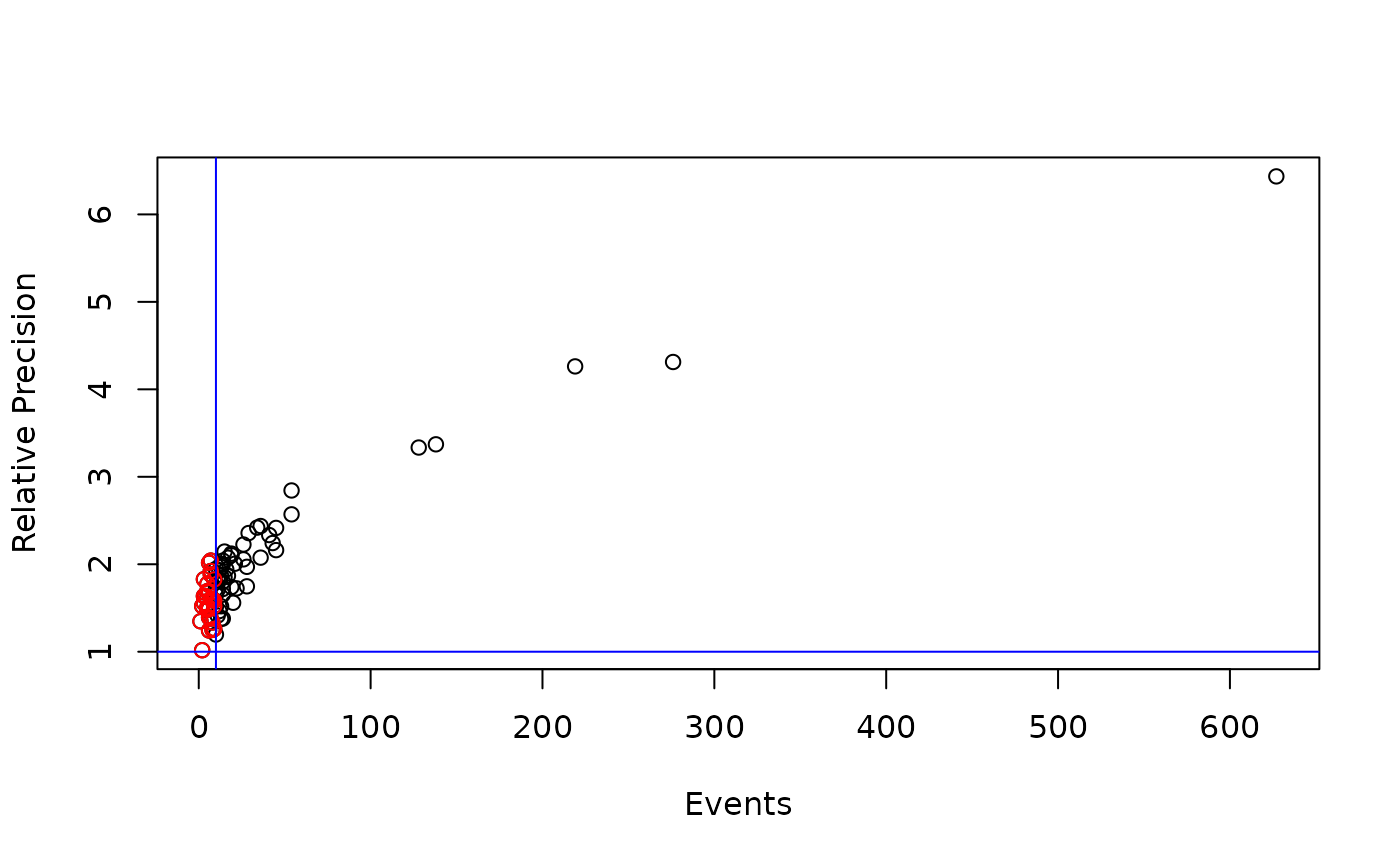

The horizontal blue line shows the relative precision cutoff, and the vertical blue line shows an event cutoff based on the suppression criteria currently used by CDC WONDER (event counts less than 10 are suppressed for privacy reasons). Red datapoints are below the population threshold but above the relative precision threshold.

This plot showcases the intense oversmoothing done by the CAR model in small-event areas. Several regions with less than 10 events (25, or 30% of our regions) have relative precisions well over the necessary threshold for reliability, despite having low event counts. Hence, we impose a threshold to prevent these estimates from being marked as reliable. However, this only fixes part of the problem: relative precisions will still be artificially inflated throughout our non-suppressed estimates, even if to a lesser degree. To address this issue, we need to stop the oversmoothing in the first place by placing a limit on model informativeness.

Model informativeness

Effectively, model informativeness quantifies the amount of ‘artificial events’ added to the model through spatial smoothing. In our example above, this resulted in 25 regions which had a sufficiently high number of events added through oversmoothing to over-inflate their relative precision.

The CAR model’s informativeness, a0, is determined by a mix of the spatial variance sig2, the non-spatial variance tau2, and the mean region rate beta for Binomially-distributed likelihoods. For Poisson-distributed likelihoods, only sig2 and tau2 determine informativeness.

The Restricted CAR (RCAR) model

RSTr features unrestricted CAR/MCAR/MSTCAR models, but also features a restricted CAR (RCAR) model which incorporates measures to prevent oversmoothing. With the RCAR model, we can limit our informativeness a0 to a ceiling, A, by tweaking the estimation process of sig2, tau2, and beta. This will ensure that our spatial smoothing does not contribute more than A events to any estimate in our model. There is an additional m0 parameter which defines a baseline number of neighbors per region. Consequently, our spatial/non-spatial variances will increase and our over-smoothing will be appropriately attenuated; this will permit the model to allow more pronounced differences between neighboring regions. Most importantly, this gives us a happy medium between no smoothing in our crude estimates and oversmoothing caused by unrestricted CAR models.

Quick et al. 2021 suggests an informativeness ceiling A of 6 and an m0 of 3 to ensure that regions with event counts less than 10 will not erroneously generate precise estimates. RSTr sets A to 6 and m0 to 3 by default.

Let’s run an RCAR model using the rcar() function, setting an informativeness ceiling of A = 6:

mod_rcar <- rcar("my_test_model", data_u, miadj, tempdir(), seed = 1234, A = 6)
#> Starting sampler on Batch 1 at Fri Dec 19 00:09:09

#> Generating estimates...
#> Model finished at Fri Dec 19 00:09:16

Notice that the traceplots for tau2 and sig2 in our restricted CAR model have significantly higher values than those in the unrestricted CAR model. This is due to the rcar model ‘blocking’ lower values and ensuring that regions don’t oversmooth. We can directly compare the two sets of results with another relative precision plot:

estimates_rcar <- get_estimates(mod_rcar)
plot(estimates_rcar$events, estimates_rcar$rel_prec, xlab = "Events", ylab = "Relative Precision", col = "purple")
points(estimates$events, estimates$rel_prec)
abline(h = 1, col = "blue")
abline(v = 10, col = "blue")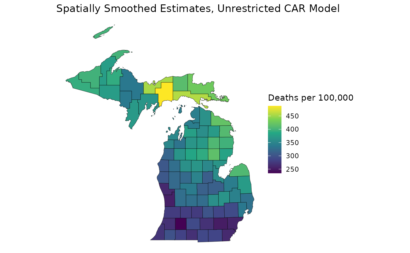

Here, the estimates for the RCAR are in purple and the estimates for the unrestricted CAR are in black. Notice how the points on the purple curve stay below the black curve at low event counts and that no purple points enter the high-precision, low-event quadrant. With A = 6, the points lie below 1 relative precision until events are greater than 10, meaning this informativeness ceiling is smoothing an ideal amount. We can also map the two estimates to visually compare the models:

library(ggplot2)
ggplot(mishp) +
  geom_sf(aes(fill = estimates$medians)) +
  labs(
    title = "Spatially Smoothed Estimates, Unrestricted CAR Model",
    fill = "Deaths per 100,000"
  ) +
  scale_fill_viridis_c() +
  theme_void()

ggplot(mishp) +
  geom_sf(aes(fill = estimates_rcar$medians)) +
  labs(
    title = "Spatially Smoothed Estimates, RCAR Model",
    fill = "Deaths per 100,000"
  ) +
  scale_fill_viridis_c() +
  theme_void()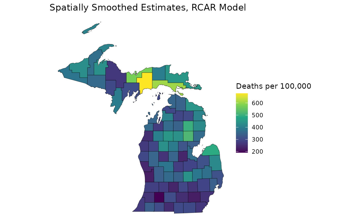

As expected, the gradient of estimates is much more sharp on the RCAR model map in comparison to the unrestricted CAR map. This is due to the decreased intensity of our spatial smoothing. Additionally, the spread of estimates for the RCAR model is wider than that of the unrestricted CAR model because of its increased spatial variance.

Restricted models and age-standardization

When age-standardizing across a CAR model, informativeness is cumulative: informativeness in individual rates when spatially smoothing will compound the informativeness in estimates age-standardized by spatially smoothed rates. Therefore, the RCAR is an excellent choice for modeling with age-standardization. Not only will individual estimates not be over-smoothed, the age-standardized estimates will benefit from enhanced reliability due to increased event counts in the crude data.

We can re-run our model with three age groups: 65-74, 75-84, and 85+. Since we are now running our models across multiple groups, we will need to extend our As to match the number of groups. Additionally, since our informativeness measures are cumulative when age-standardizing, we should split our A = 6 informativeness ceiling among all of our groups of interest. If we want, we can weight each group’s A by their total events:

data_u <- lapply(miheart, \(x) x[, c("65-74", "75-84", "85+"), "1988", drop = FALSE])
A <- 6 * colSums(data_u$Y) / sum(data_u$Y)
mod_rcar <- rcar("test_rcar", data_u, miadj, tempdir(), seed = 1234, A = A)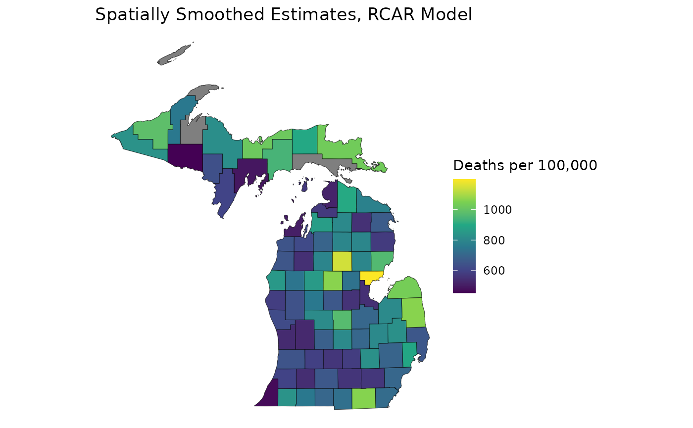
#> Starting sampler on Batch 1 at Fri Dec 19 00:09:17

#> Generating estimates...
#> Model finished at Fri Dec 19 00:09:24

While our individual groups will have lower relative precisions due to lower respective As, when we age-standardize, we will have the same effective smoothing power as our singular A = 6 restricted model:

std_pop <- c(68775, 34116, 9888)
mod_rcar <- age_standardize(mod_rcar, std_pop, "65up")
est_rcar <- get_estimates(mod_rcar)
ggplot(mishp) +
  geom_sf(aes(fill = est_rcar$medians)) +
  labs(
    title = "Age-Standardized Spatially Smoothed Estimates, RCAR Model",
    fill = "Deaths per 100,000"
  ) +
  scale_fill_viridis_c() +
  theme_void()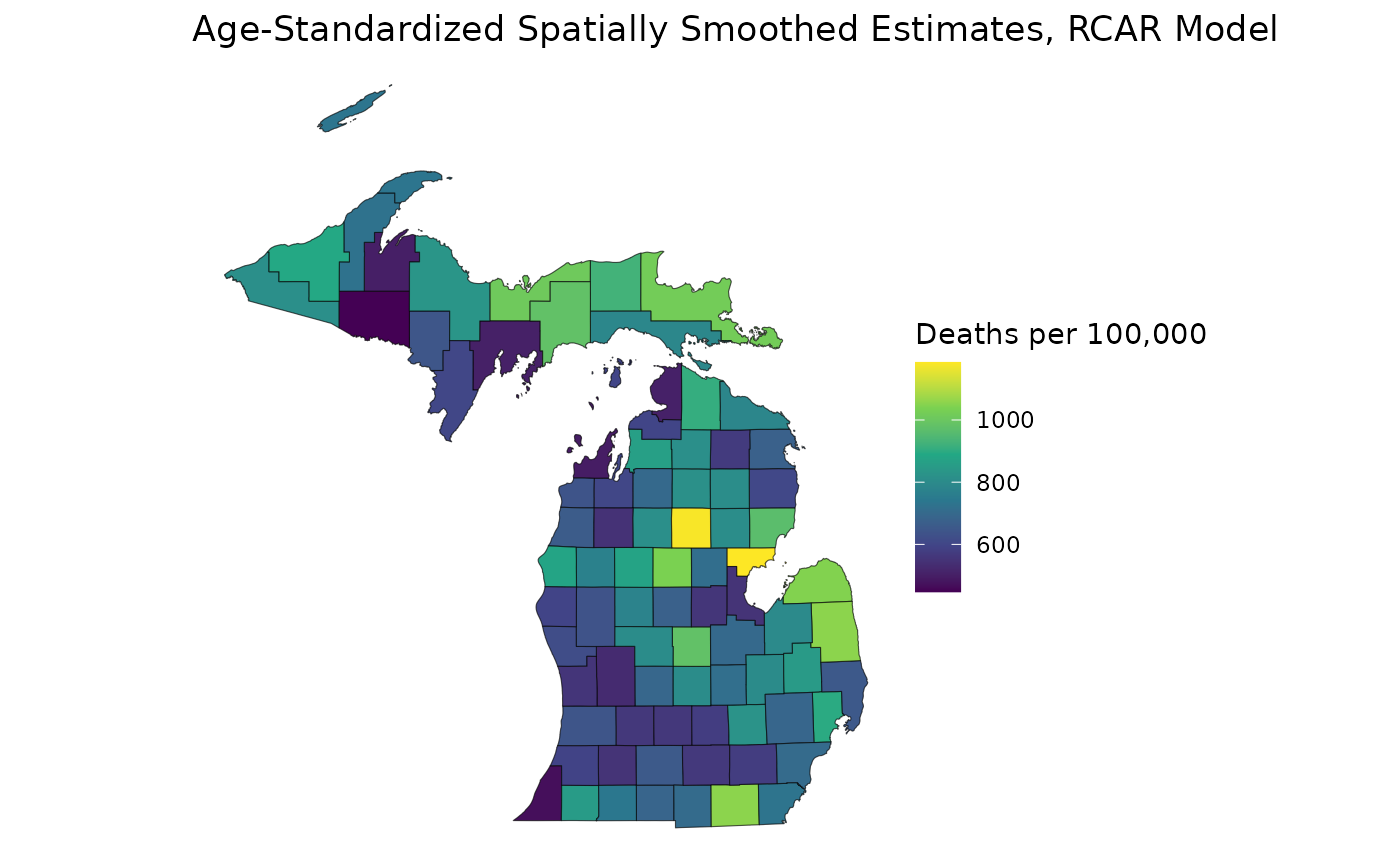

The RCAR Model, Reliability, and Suppression

Remember that for unrestricted CAR models, we have to impose an additional event/population threshold for reliability to capture high-precision estimates in low-event areas. As we saw in the event/relative precision plot, these thresholds are no longer necessary when we suppress our estimates with an RCAR model:

mod_rcar <- suppress_estimates(mod_rcar)
est_rcar <- get_estimates(mod_rcar)
ggplot(mishp) +
  geom_sf(aes(fill = est_rcar$medians_suppressed)) +
  labs(
    title = "Spatially Smoothed Estimates, RCAR Model",
    fill = "Deaths per 100,000"
  ) +
  scale_fill_viridis_c() +
  theme_void()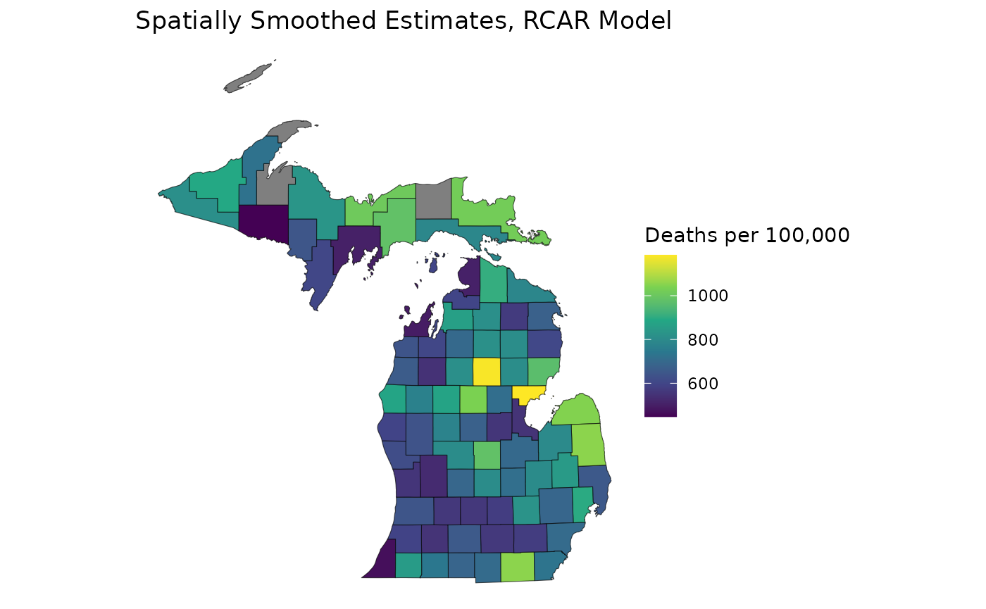

With the RCAR model, we get the benefit of age-standardizing our spatially smoothed estimates without the compounded oversmoothing from unrestricted models.

Choosing between restricted vs unrestricted models

Now that we’ve elucidated the benefits of using restricted models, we can work through the most appropriate use case for each model:

The RCAR model is virtually always preferred to the unrestricted CAR model. If you are not interested in temporal trends or group/time interactions, the RCAR will likely be your best option, particularly if you are age-standardizing.
The MCAR model is useful if you are specifically interested in interactions between sociodemographic groups and don’t have temporal data.
The MSTCAR model is the best option when investigating linear trends in temporal data or if you are specifically interested in interactions between sociodemographic groups across time. If your trends depict multiple behaviors, it is recommended to either run two MSTCAR models with separate time periods for each trend or to run concurrent RCAR models. Note that all *car() functions accept up to three-dimensional arrays and will concurrently run models for different groups/time periods if necessary.

Future developments

Restricted models for MCAR and MSTCAR continue to be under development. Development for a restricted Univariate Spatiotemporal CAR (STCAR) model is also underway. RSTr will incorporate these restricted models as they become available.

Final thoughts

In this vignette, we investigated model informativeness and the tendency of unrestricted BYM models to oversmooth estimates, along with some benefits of restricted CAR models. This vignette concludes the main sections on using the functions in the RSTr package. After reading these, you should be able to prepare your event and adjacency data, choose and configure your model as necessary, age-standardize estimates, and determine which estimates are reliable. If you are interested in the more advanced features of the RSTr involving sample processing, read vignette("RSTr-samples"); if you’d like more information on defining custom inits and priors, check vignette("RSTr-initialvalues") and vignette("RSTr-priors"), respectively; if you are interested in learning more about how RSTr’s models work, read vignette("RSTr-models").