02: Understanding and Preparing Your Adjacency Structure • RSTr

Overview

The adjacency structure is a set of instructions that show the spatial relationship between each region and informs RSTr which counties to pull information from when spatially smoothing. In this vignette, we will cover the requirements for the adjacency object along with walking through the setup of the adjacency information.

Requirements

Adjacency information is input as a list adj where each element adj[[i]] is a vector of indices denoting regions that are neighbors of region i. Below, we will walk through the construction of the adjacency information and address common issues that may arise.

Example: Massachusetts Map Data

For this example, we will continue using Massachusetts data as we did in section 2. Included is an example dataset that contains Massachusetts shapefile information, generated using the tigris package:

head(mamap)

This dataset contains several variables related to Census information on Massachusetts, but for our purposes we are only interested in two variables:

GEOID contains the FIPS code for each county. We can use this to associate each county with the counties in our event/population data; and
geometry describes how to map each region. We can use this to generate our adjacency information.

To begin, let’s first arrange mamap by GEOID to ensure the counties are in the same order as our maexample data, then generate some adjacency information using the spdep package:

ma_shp <- sf::st_as_sf(mamap[order(mamap$GEOID), ])
ma_adj <- spdep::poly2nb(ma_shp)
#> Warning in spdep::poly2nb(ma_shp): some observations have no neighbours;
#> if this seems unexpected, try increasing the snap argument.
#> Warning in spdep::poly2nb(ma_shp): neighbour object has 3 sub-graphs;
#> if this sub-graph count seems unexpected, try increasing the snap argument.

spdep::poly2nb() takes the information in ma_shp$geometry and looks for any regions with touching boundaries (i.e., queen contiguity). ma_adj is a list that contains the indices of each region that is a neighbor with a given region. Looking at ma_adj gives us some more information:

ma_adj
#> Neighbour list object:
#> Number of regions: 14 
#> Number of nonzero links: 38 
#> Percentage nonzero weights: 19.38776 
#> Average number of links: 2.714286 
#> 2 regions with no links:
#> 1252, 1577
#> 3 disjoint connected subgraphs

ma_adj tells that there are 14 regions linked in 38 unique ways. However, it also notes that there are two regions with no links. Regions with no links are problematic for RSTr because it has no information with which to spatially smooth, causing the model to crash. Because our data is in this incomplete format, we will have to do some investigation and fixing to get it ready for use.

Let us first look at the dataset to see which counties have no neighbors. ma_adj tells us that regions 4 and 10 are our regions with no links, but we can also use spdep::card() to give us the indices of our no-link counties:

no_neigh <- spdep::card(ma_adj) == 0

We can now investigate ma_shp for the counties with no neighbors:

ma_shp[no_neigh, ]
#> Simple feature collection with 2 features and 12 fields
#> Geometry type: MULTIPOLYGON
#> Dimension:     XY
#> Bounding box:  xmin: -70.95137 ymin: 41.23796 xmax: -69.96018 ymax: 41.52178
#> Geodetic CRS:  NAD83
#>      STATEFP COUNTYFP COUNTYNS       AFFGEOID GEOID      NAME         NAMELSAD
#> 1252      25      007 00606930 0500000US25007 25007     Dukes     Dukes County
#> 1577      25      019 00606936 0500000US25019 25019 Nantucket Nantucket County
#>      STUSPS    STATE_NAME LSAD     ALAND     AWATER
#> 1252     MA Massachusetts   06 267292993 1004291414
#> 1577     MA Massachusetts   06 119637319  666826424
#>                            geometry
#> 1252 MULTIPOLYGON (((-70.8071 41...
#> 1577 MULTIPOLYGON (((-70.23405 4...

According to this, our two no-link counties are Dukes and Nantucket (FIPS 25007 and 25019, respectively). Let’s check out a ggplot of our data to further investigate:

library(ggplot2)

ggplot(mamap) +
  geom_sf(aes(fill = NAME)) +
  geom_sf_label(aes(label = NAME))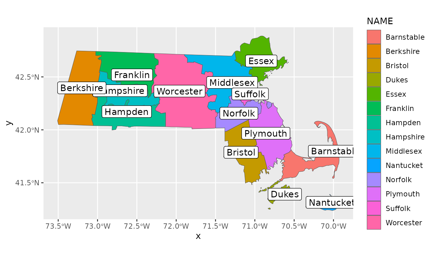

Here, we’ve generated a map colored by region and labeled with the name of each county. We can see Dukes and Nantucket in the southeast corner, and if you zoom in, you can see that these two counties aren’t touching any other counties. Upon closer inspection, Barnstable County seems like a good contender for a neighbor to both Dukes and Nantucket County; Dukes and Nantucket County are also close enough to be neighbors to each other. To rectify this, we can make some changes to our adjacency information. Let’s first get a feel for which counties are associated with which indices:

county_key <- seq_along(ma_shp$NAME)
names(county_key) <- ma_shp$NAME
county_key
#> Barnstable  Berkshire    Bristol      Dukes      Essex   Franklin    Hampden 
#>          1          2          3          4          5          6          7 
#>  Hampshire  Middlesex  Nantucket    Norfolk   Plymouth    Suffolk  Worcester 
#>          8          9         10         11         12         13         14

We can see that Barnstable has an index of 1, Dukes has an index of 4, and Nantucket has an index of 10. We can use the add_neighbors() function to set these counties as mutual neighbors:

ma_adj <- add_neighbors(ma_adj, c(1, 4, 10))

Now if we look at ma_adj, the message about no-link regions is gone.

Finally, even though we connected the two island counties to the mainland counties of MA, as long as each region has at least one neighbor, it is usable within RSTr. This means that, theoretically, we could have made just Dukes and Nantucket neighbors of each other, creating two separate islands with no related neighbors. In this case, every region on both islands still has at least one neighbor.

Closing Thoughts

In this vignette, we used spdep::poly2nb() to generate our adjacency structure. We then fixed issues with counties without neighbors and applied a naming scheme to the adjacency information consistent with the data object created in section 2. From here, the model is ready to be run with our data and adjacency information!