An Introduction to the RSTr Package • RSTr

Overview

RSTr is an R package that provides a host of Bayesian spatiotemporal models in conjunction with Rcpp to quickly and easily generate spatially-smoothed age-standardized estimates for your spatial data. This vignette introduces you to the basics of the RSTr package and shows you how to apply the basic functions to the included example data in a three-step workflow to get small area estimates: (1) data preparation, (2) running the model, and (3) extracting and post-processing estimates.

Models

The models provided in the RSTr package are based on the Besag, York, and Mollié (1991) Conditional Autoregressive (CAR) model, which spatially smooths data by incorporating information such as event and population counts from neighboring geographic units (counties, census tracts, etc.). The degree of spatial smoothing is determined by a spatial region’s respective population size. These spatially smoothed estimates are generated based on the posterior samples generated in an MCMC algorithm. The CAR model can be extended to several levels of complexity, depending on the input data:

BYM CAR (CAR): Spatially smooths across geographies;
Restricted CAR (RCAR): Spatially smooths across geographies and prevents over-smoothing;
Multivariate CAR (MCAR): Spatially smooths across geographies and sociodemographic groups; and
Multivariate Spatiotemporal CAR (MSTCAR): Spatially smooths across geographies, sociodemographic groups, and time periods.

For this vignette, we will demonstrate RSTr’s functionality with an MSTCAR model.

Example workflow with the MSTCAR model

The process of generating estimates with RSTr can be separated into three main steps: data preparation, model running, and estimate extraction. In the following section, we will work through each step one-by-one, using example data provided with RSTr. Here is a chart describing the three steps of the workflow:

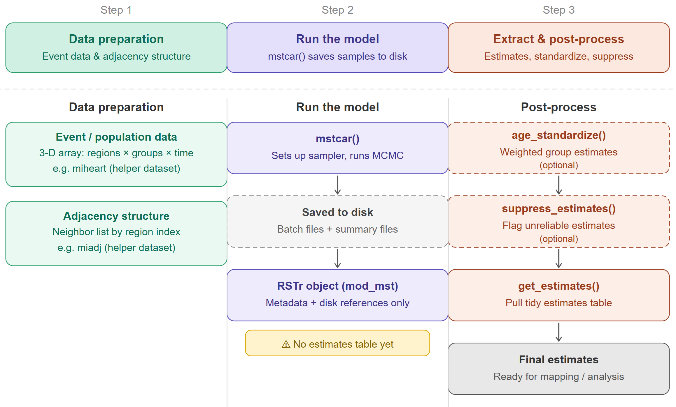
Data preparation

Models with RSTr take, at a minimum, two pieces of data: event/population data, and adjacency information. Event and population data are packaged into a single list object, and the adjacency information is a neighbors list based on contiguous boundaries.

Event/population data

RSTr requires event counts for a parameter of interest, stratified by region, group, and time period, and its corresponding population counts. Event/population data must be organized in a very specific manner. RSTr’s models can accept up to three-dimensional arrays: in the MSTCAR model, for example, spatial regions must be on the rows, socio/demographic groups must be on the columns, and time periods must be on the matrix slices. In the current version of RSTr, universal data is required - the models are not yet designed to handle survey data.

RSTr includes miheart, a helper dataset included with RSTr for demonstration purposes. When running your own analysis, you will substitute this with your own event/population data structured in the same format. miheart is binomial-distributed myocardial infarction deaths in six age groups from 1979-1988 in Michigan. Reference miheart to see how this data looks or ?miheart for more information on the dataset.

For more information on preparing your event data, read vignette("RSTr-event")

Adjacency information

The adjacency information is a list that tells RSTr which regions are neighbors of one other based on their region index (i.e., the order they appear in the dataset). Every region must have at least one neighbor. The adjacency structures must be listed in the same order as your count data. The easiest way to generate this adjacency information is through the spdep::poly2nb() function.

RSTr includes miadj, a helper dataset included with RSTr for demonstration purposes. When running your own analysis, you will substitute this with an adjacency structure derived from your own shapefile, for example using spdep::poly2nb(). For more information on preparing your adjacency data, read vignette("RSTr-adjacency").

Running the model

RSTr’s *car() functions create an RSTr model object which contains all the information needed to run a model, such as the number of iterations, the model type, the current sample value, etc. This model object is periodically saved into a model folder name, which lives under the directory dir. As the models run, the MCMC samples are also saved in the model folder. A random seed can also be specified directly within the *car() functions for replicability purposes.

With our data set up and a knowledge of the basic components of the *car() functions, we can run our first model. Let’s use the provided Michigan example data, miheart and mishp:

mod_mst <- mstcar(
  name = "my_test_model",
  data = miheart,
  adjacency = miadj,
  dir = tempdir(),
  seed = 1234
)

Here, we use the mstcar() function to specify our model. mstcar() accepts a few different arguments:

The name argument specifies the folder where the model data lives;
The data argument specifies event/population data;
The adjacency argument specifies our adjacency structure;
The dir argument specifies the directory where to save the folder; and
The seed argument specifies the random seed.

mstcar() sets up the sampler, runs 6,000 MCMC iterations in 60 batches of 100, and saves the results locally inside the folder specified by dir/name (e.g., tempdir()/my_test_model). Samples are not held in RAM because large MSTCAR models can exceed available memory.

The mod_mst object created in your R environment does not contain a table of estimates. Instead, it stores model metadata (name, type, number of samples, etc.) and references to where the samples and summaries are saved on disk.

Note that mstcar() accepts more arguments than are used here, but these are the only ones needed to get started. Priors and initial values, for example, can be specified manually, but this is outside the scope of this vignette. There will also be checks performed on the input data: if something is wrong, warnings and error messages will tell you what is wrong and how to fix it. For a list of diagnostic errors and what they mean, read vignette("RSTr-troubleshooting").

Console outputs will show the current batch number, the progress within that batch, and the elapsed time. The model Rds file will be updated as the sampler progresses in case you need to reload your model at a later date. If the model crashes for any reason or R closes while the model is being run, the model Rds file will keep track of the current batch and pick back up where it left off when re-run. While mstcar() is running, the R plot window will show traceplots from a selection of estimates to check stability and diagnose any potential issues.

mstcar() takes care of the vast majority of model preparation: within the function, the model is set up, samples are generated, and our medians are estimated. Once the function finishes, we can get an overview of our model:

mod_mst
#> RSTr object:
#> 
#> Model name: my_test_model 
#> Model type: MSTCAR 
#> Data likelihood: binomial 
#> Estimate Credible Interval: 95% 
#> Number of geographic units: 83 
#> Number of samples: 6000 
#> Estimates age-standardized: No 
#> Estimates suppressed: No

Here, we get a birds-eye-view of the model, including the model we used (MSTCAR), the data likelihood type, the number of geographic units, and whether our estimates have been age-standardized or suppressed along reliability criteria.

Note that running mstcar() does not produce a ready-to-use table of estimates in memory. mstcar() only sets up the sampler, runs it, and saves raw samples and summaries to disk. Estimates must be extracted using the get_estimates() function described in the following section.

If you want to learn more about mstcar() and the other model functions, read vignette("RSTr-car").

Estimate extraction

Now that we’ve run the mstcar() function, how do we get our estimates? The estimates are saved to disk and referenced by mod_mst, but because this object also holds all information related to the model, we have to extract the estimates specifially using other RSTr functions.

With the get_estimates() function, we can get a more detailed look at our estimates. For this type of mortality data, it is common to observe the rates per 100,000 population, so we set the rates_per argument in get_estimates() to 1e5:

mst_estimates <- get_estimates(mod_mst, rates_per = 1e5)
head(mst_estimates)
#>   county group year  medians ci_lower  ci_upper  rel_prec events population
#> 1  26001 35-44 1979 44.02662 30.63858  67.32566 1.2000580      1        964
#> 2  26003 35-44 1979 76.91252 54.16346 140.01402 0.8958884      1       1011
#> 3  26005 35-44 1979 20.95290 15.13452  27.64008 1.6754864      0       9110
#> 4  26007 35-44 1979 34.91586 20.06479  47.20547 1.2864766      0       3650
#> 5  26009 35-44 1979 35.72440 22.58465  53.36119 1.1607673      0       1763
#> 6  26011 35-44 1979 50.38792 34.86763  77.69188 1.1766211      0       1470

The mst_estimates object contains in-depth information about our model estimates, including the medians, the credible intervals, the relative precisions, and the event/population counts; region, group, and time period columns are also provided.

Age-standardization

One of the most important features of the RSTr package is the ability to easily generate age-standardized estimates. Let’s say we want to get age-standardized estimates for the 35-64 age group; for our model, we use the age_standardize() function, then specify the groups of interest, their associated standard populations, and the name we want to give them. Since we are using data from 1979-1988, we can use 1980 standard populations from NIH to generate a std_pop standard population vector:

std_pop <- c(68775, 34116, 9888)
mod_mst <- age_standardize(mod_mst, std_pop, new_name = "35-64", groups = c("35-44", "45-54", "55-64"))
mod_mst
#> RSTr object:
#> 
#> Model name: my_test_model 
#> Model type: MSTCAR 
#> Data likelihood: binomial 
#> Estimate Credible Interval: 95% 
#> Number of geographic units: 83 
#> Number of samples: 6000 
#> Estimates age-standardized: Yes 
#> Age-standardized groups: 35-64 
#> Estimates suppressed: No

Notice now that the mod_mst object indicates we have age-standardized our estimates and the names of our age-standardized groups.

mst_estimates_as <- get_estimates(mod_mst)
head(mst_estimates_as)
#>   county group year   medians  ci_lower  ci_upper rel_prec events population
#> 1  26001 35-64 1979 107.21691  83.59800 129.46863 2.337376      7       3353
#> 2  26003 35-64 1979 186.94283 151.41174 248.32560 1.928959     12       3105
#> 3  26005 35-64 1979  64.54074  54.69219  74.28448 3.294192     27      23926
#> 4  26007 35-64 1979  84.66275  66.41816  99.32165 2.573063     15      10000
#> 5  26009 35-64 1979  88.90282  68.02031 107.23080 2.267322     11       5152
#> 6  26011 35-64 1979 120.13771  98.89313 153.58019 2.196822      8       4517

Now, get_estimates(mod_mst) shows the age-standardized estimates. Should you want to see those instead, you can set the argument standardized = FALSE.

Estimate suppression

While the main benefit of RSTr is generating reliable estimates from small-population areas, we cannot guarantee that all estimates generated by mstcar() will be reliable. Therefore, it is prudent to suppress estimates that are deemed unreliable. For MSTCAR models, we can use two criteria to test for reliability: relative precision (i.e., the ratio of the median estimate to the width of its credible interval) and population count. For relative precisions, we aim for a value of at least 1 (i.e., the median is larger than the width of its credible interval), and for myocardial infarction death rates, we typically aim for a population threshold of at least 1,000. Using the suppress_estimates() function, we can generate suppressed estimates for our age-standardized rates:

mod_mst <- suppress_estimates(mod_mst, threshold = 1e3)
mod_mst
#> RSTr object:
#> 
#> Model name: my_test_model 
#> Model type: MSTCAR 
#> Data likelihood: binomial 
#> Estimate Credible Interval: 95% 
#> Number of geographic units: 83 
#> Number of samples: 6000 
#> Estimates age-standardized: Yes 
#> Age-standardized groups: 35-64 
#> Estimates suppressed: Yes 
#> Number of reliable age-standardized rates: 817 / 830 (98.4%)
mst_estimates_as <- get_estimates(mod_mst)
head(mst_estimates_as)
#>   county group year   medians medians_suppressed  ci_lower  ci_upper rel_prec
#> 1  26001 35-64 1979 107.21691          107.21691  83.59800 129.46863 2.337376
#> 2  26003 35-64 1979 186.94283          186.94283 151.41174 248.32560 1.928959
#> 3  26005 35-64 1979  64.54074           64.54074  54.69219  74.28448 3.294192
#> 4  26007 35-64 1979  84.66275           84.66275  66.41816  99.32165 2.573063
#> 5  26009 35-64 1979  88.90282           88.90282  68.02031 107.23080 2.267322
#> 6  26011 35-64 1979 120.13771          120.13771  98.89313 153.58019 2.196822
#>   events population
#> 1      7       3353
#> 2     12       3105
#> 3     27      23926
#> 4     15      10000
#> 5     11       5152
#> 6      8       4517

mod_mst now shows us that our estimates are suppressed and indicates the number of reliable rates.

If you want to learn more about get_estimates(), age_standardize(), and suppress_estimates(), read vignette("RSTr-estimates").

Illustrative Example: Mapping Estimates

We can get a better picture of the geographic patterns in our data with a map. Using ggplot (or your favorite mapping package), Let’s see how the (non-age-standardized) estimates were smoothed:

# Original Myocardial Infarction Death Rates in MI, Ages 35-64, 1988
estimates_88 <- mst_estimates_as[mst_estimates_as$year == "1988", ]
estimates_3564 <- estimates_88[estimates_88$group == "35-64", ]
raw_3564 <- (estimates_3564$events / estimates_3564$population * 1e5)
ggplot(mishp) +
  geom_sf(aes(fill = raw_3564)) +
  labs(
    title = "Raw Myocardial Infarction Death Rates in MI, Ages 35-64, 1988",
    fill = "Deaths per 100,000"
  ) +
  scale_fill_viridis_c() +
  theme_void()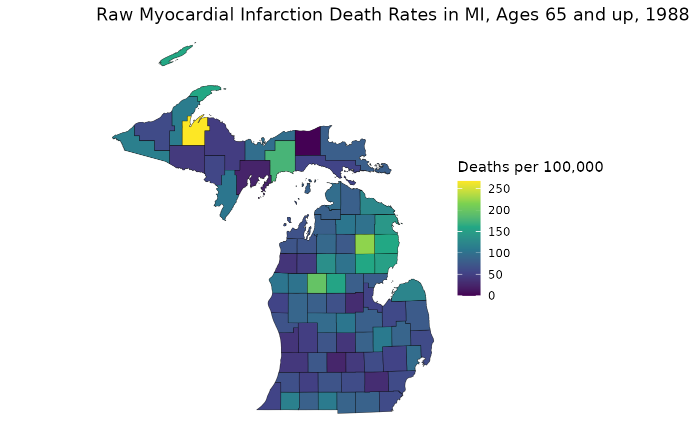

# Spatially Smoothed MI Death Rates in MI
est_3564 <- estimates_3564$medians
ggplot(mishp) +
  geom_sf(aes(fill = est_3564)) +
  labs(
    title = "Smoothed Myocardial Infarction Death Rates in MI, Ages 35-64, 1988",
    fill = "Deaths per 100,000"
  ) +
  scale_fill_viridis_c() +
  theme_void()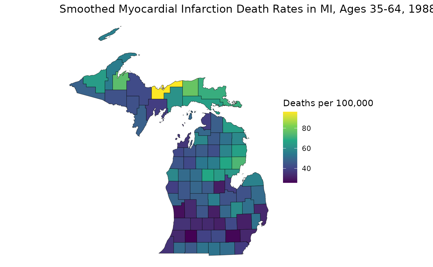

This map helps us see how RSTr smooths rates. First, notice how the range of the two plots are different: the smoothed map has a smaller range because RSTr stabilizes high and low extreme values which are usually caused by low population counts. Also, notice how the transitions between high-rate and low-rate regions are more gradual on the smoothed map. This is a consequence of using neighboring regions to inform and stabilize estimates.

From here, we can get a better idea of how these maps contrast. For example, on the first map, the largest region of interest is the middle portion of the Lower Peninsula (LP), but on the smoothed map, much of this area has attenuated rates. On the flip side, many areas in the Upper Peninsula (UP) have relatively lower rates on the first map, but we can see on the smoothed map that the highest rate in the state is in the UP. The higher-rate areas on the LP are focused around counties on Saginaw Bay in the east, indicating that these areas may require more attention than previously thought. These are the kinds of inferences that can be made using estimates generated by the RSTr package and the main motivation for running this spatiotemporal model.

Closing Thoughts

This vignette introduces you to inputting data into the mstcar() function, extracting estimates with the get_estimates() function, age-standardizing estimates with the age_standardize() function, suppressing estimates with the suppress_estimates() function, and finally making a map with estimates gathered from get_estimates() function. What we’ve discussed here is just scratching the surface of the RSTr package. Other package vignettes will dive deeper into the intricacies of each component of the package. All of these things together will ensure you get the most out of using RSTr.